

How To Clear Scratchpad On Ti-nspire Cx Ii
Graphing with the Scratchpad
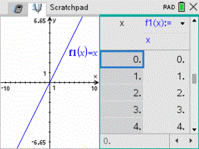
| one. | Press » to open the Scratchpad Graph page if information technology is non already open. |
By default, the entry line is displayed. The entry line displays the required format for typing a relation. The default graph blazon is Part, so the form f1(x)= is displayed.
If the entry line is not shown, press or printing btwo3 to display the entry line and blazon an expression to graph.
| 2. | Press b > Graph Entry/Edit and select a graph type. |
For instance:
| • | To graph an equation for a circle, press b > Graph Entry/Edit > Equation > Circle > (10-h) 2 + (y-one thousand) two = r 2 or press b3231. Fill in the equation and printing · to draw the circumvolve. |
| • | To graph a function, press b > Graph Entry/Edit > Role or press b3ane. |
The entry line changes to brandish the expression format for the specified graph type. You can specify multiple relations of each graph type.
| 3. | Blazon an expression and any other parameters required for the graph type. |

| 4. | Press · to graph the relation, or press ¤ to add another relation. If necessary, you lot can use printing b4 to choose a tool on the Window/Zoom menu and adjust the viewing expanse. |
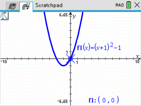
When yous graph the relation, the entry line disappears to show an uncluttered view of the graph. If you select or trace a plot, the relation that defines the plot is displayed on the entry line. Y'all can modify a plot by defining a relation or by selecting and changing the graph.
As you graph multiple plots, the defining relation is displayed for each. You lot can define and graph a maximum of 99 relations of each type.
| 5. | Use the b key to explore and analyze the relation to: |
| • | Trace the relation. |
| • | Observe points of interest. |
| • | Assign a variable in the expression to a slider. |
Viewing the Table
| ▶ | To display a table of values respective to the electric current plots, press b > Tabular array > Split-screen Table (bvii1). |
| ▶ | To hide the tabular array, click the graph side of the carve up screen, and then printing b > Table > Remove Table (b7two). Yous can besides press Ctrl + T. |
| ▶ | To resize columns, click the table and press b > Actions > Resize (b1ane). |
| ▶ | To delete a cavalcade, edit an expression, or edit tabular array settings, click the table and press b > Tabular array (b 2). |
Changing the Advent of the Axes
As you work with graphs, the Cartesian axes are displayed by default. Yous can alter the appearance of the axes in the following means:
| i. | Press b4 and choose the Zoom tool to use. |
| 2. | Select the axes and press /bii to activate the Attributes tool. |
| a) | Press £ or¤ to move to the attribute to change. For instance, choose the cease way attribute. |
| b) | Press ¡ or¢ to choose the way to apply. |
| c) | Alter whatsoever other attributes of the axes equally required for your piece of work, and then press · to exit the attributes tool. |
| three. | Adapt the axes scale and tic mark spacing manually. |
| a) | Click and concord 1 tick mark, and move information technology on the axis. The spacing and number of tic marks increases (or decreases) on both axes. |
| b) | To arrange the scale and tic mark spacing on a single axis, press and concord thousand, and and so grab and drag a tic mark on that axis. |
| four. | Modify axis cease values by double-clicking them and typing new values. |
| 5. | Adjust the location of the axes. To movement the existing axes without resizing or rescaling them, click in and drag an empty region of the screen until the axes are in the desired location. |
| vi. | Change the axes' scales by pressing b > Window/Zoom > Window Settings (b4i). |
Blazon the values of your choice over the current values for x-min, x-max, y-min, y-max, Xscale, and Yscale and click .
| 7. | Press b > View > Hide Axes (btwoone) to hide or show the axes. |
| • | If the axes are shown on the folio, selecting this tool hides them. |
| • | If the axes are hidden on the page, selecting this tool redisplays them. |
Tracing a Plot
Graph Trace moves through the points of a graphed function, parametric, polar, sequence, or scatter plot. To enable the trace tool:
| ane. | Press b > Trace > Graph Trace (bv1) to move across the plot in Trace way. |
| 2. | (Optional) To modify the trace step increment for tracing, press b53. |
Subsequently y'all blazon a different stride increment, the Graph Trace tool moves beyond the graph in steps of that size.
| iii. | Employ Graph Trace to explore a plot in the post-obit ways: |
| • | Motion to a indicate and hover to move the trace cursor to that indicate. |
| • | Press ¡ or¢ to move from point to bespeak on the office's graph. The coordinates of each point traced are displayed. |
| • | Press £ or¤ to move from i plot to another. The point'south coordinates update to reflect the new location of the trace. The trace cursor is positioned on the point of the new graph or plot with the closest x value to the last point identified on the previously traced function or graph. |
| • | Blazon a number and press · to move the trace cursor to the point on the plot with contained coordinates nearest the typed value. |
| • | Create a persistent bespeak that remains on the graph past pressing · when the trace signal reaches the point you want to characterization. The point remains after you exit Graph Trace mode. |
Notes:
| • | The string undef is displayed instead of a value when yous move over a indicate that is not defined for the office (a discontinuity). |
| • | When you trace beyond the initially visible graph, the screen pans to bear witness the expanse being traced. |
| 4. | Press d or choose another tool to exit Graph Trace. |
Finding Points of Interest
You lot can utilise the tools on the menu to find a point of involvement in a specified range of any graphed office. Cull a tool to find zero, the minimum or maximum, the bespeak of intersection or inflection, or the numeric derivative (dy/dx) or Integral on the graph.
| one. | Select the point of interest that you lot desire to find on the Analyze Graph card. For example, to find a zero, printing b61. |
| non-CAS and Verbal Arithmetics | CAS | |
|---|---|---|
| Zero | b61 | bvi1 |
| Minimum | bvi2 | bhalf-dozen2 |
| Maximum | bhalf-dozen3 | b63 |
| Intersection | bsixiv | b6four |
| Inflection | Non applicable | b65 |
| dy/dx | bhalf-dozen5 | b66 |
| Integral | b66 | b67 |
| Analyze Conics | b67 | b68 |
The icon for the selected tool is displayed at the top left on the work area. Signal to the icon to view a tooltip about how to employ the selected tool.
| 2. | Click the graph you want to search for the point of involvement, and then click a second time to indicate where to starting time the search for the point. |
The 2d click marks the lower leap of the search region and a dotted line is displayed.
Note: If yous are finding the derivative (dy/dx), click the graph at the point (numeric value) to use for finding the derivative.
| three. | Press ¡ or ¢ to move the dotted line that marks the search region, and so click the signal at which you want to stop the search (upper spring of the search region). |
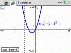
| 4. | Press · at the point to start the search. The tool shades the range. |
If the search region you specified includes the point of interest, a label for the point is displayed. If you lot change a graph that has points of involvement identified, be sure to check for changes in points of interest. For example, if you edit the function on the entry line or dispense a plot, the indicate where the graph intersects zippo tin modify.
The labeled points of interest remain visible on the graph. You tin can exit the tool by pressing d or choosing some other tool.
Source: https://education.ti.com/html/webhelp/EG_TINspire/EN/content/m_scratchpad/sc_graphing_with_the_scratchpad.HTML
0 Response to "How To Clear Scratchpad On Ti-nspire Cx Ii"
Post a Comment